Introduction:
In this assignment, we will be using rasters to create graphs. Raster data consists of a matrix of cells or pixels organized into a grid, where each cell/pixel represents a value of something that can be measured, such as temperature. This is where mapmaking gets involved in R, because raster data can be overlaid on a map, meaning shapefiles and other geographic data gets involved here. We will need special packages for this assignment, and you ought to download them if you don't already have them if you want to do this assignment yourself. In this assignment, the following packages will be used: raster, rasterVis, rgdal, RColorBrewer, and latticeExtra.
About NDVI:
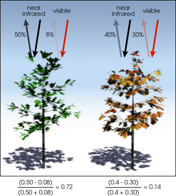
For this assignment, we will be creating a graph of the Normalized Difference Vegetation Index (NDVI) of the Great Plains region from 2001 to 2016. This is a vegetation index indicative of the density and "greenness" of vegetation. NDVI is found by finding the difference between near-infrared radiation (which vegetation strongly reflects) and visible red light (which is absorbed by vegetation) found by a remote sensor that is flown above the study area in a plane. Here's the formula for finding NDVI where NIR represents near-infrared radiation and VIS represents visible red light:

Don't get too worried about NIR and VIS, because the remote sensor will find those values for you. NDVI ranges in value from -1 to 1, in which the more positive values represent lusher, greener, denser vegetation cover. A lower NDVI is indicative of sparser or dead vegetation. Here's a little table for reference.
| NDVI Value | Cover Type | Possible Environment |
|---|---|---|
| NDVI < 0 | water, snow, or clouds | ocean, icecaps |
| 0 < NDVI < 0.2 | rock, sand, concrete | barren, urban, desert, mountains |
| 0.2 < NDVI < 0.5 | shrubs, grasslands, crops, dying vegetation | farmland, prairie, steppe, savanna, drought area |
| 0.5 < NDVI < 0.9 | trees, fully grown crops, healthy vegetation | farmland, temperate forests |
| 0.9 < NDVI < 1 | tropical plants, large trees, lush vegetation | swamps, wetlands, rainforests |
Creating the Graphs:
As always, remember to set the directory to the folder you are storing the files you want to access in, and remember to load each package you will be using using the library() command. We will be using the file MAX_0116_MEAN.tif file for this, and lay it over the shapefile lower48.shp that represents the 48 continental United States. Thanks to the packages we installed, actually plotting the data is a breeze. It's working with it and touching up the graph that's going to be the harder part of this assignment. We store our .tif file into a variable I'll call dem and the shapefile into a variable I'll call conus. Here's the code:
> library(latticeExtra)
> library(raster)
> library(rasterVis)
> library(rgdal)
> library(RColorBrewer)
> dem <- raster("MAX_0116_MEAN.tif")
> theme <- rasterTheme(region = brewer.pal("BrBG", n=11))
> graph <- levelplot(dem, margin = list(FUN = "median"), main = "Maximum NVDI 2001-2016 \n American Great Plains", xlab="Easting Coordinate (m)", ylab="Northing Coordinate (m)", par.setting = theme)
> shp <- readOGR(".", "lower48")
> graph <- graph + layer(sp.lines(shp, col = "black", lwd = 0.5))
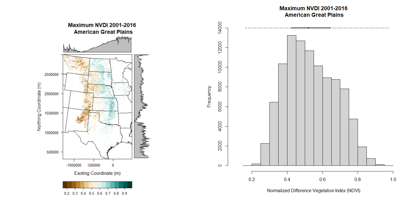
In case you want to know, the coordinate system used here is the Universal Transversal Mercator (UTM) coordinate system. As long as you can tell where the data is from the shapefile, we shouldn't have to worry too much about a coordinate system most people have never heard of. Also, the term for what we created is called a levelplot. We're also going to create a histogram with a boxplot on it. Here's the code for that, as well as our two final products below:
> hist(dem, freq = TRUE, main="Maximum NVDI 2001-2016\n American Great Plains", xlab = "Normalized Difference Vegetation Index (NDVI)", xlim = c(0.1,1), ylim = c(0, 14000))
> boxplot(dem, horizontal = TRUE, at = 14000, add = TRUE, axes = FALSE, boxwex = 200)
Analysis:
There exists a clear, decreasing gradient in maximum NDVI values for the time period studied as you go from east to west across the Great Plains. This is not surprising, because there is also a precipitation gradient that follows in lockstep with the NDVI gradient. The 100th Meridian passes through this region, which separates the wetter eastern half of the United States from the drier western half. NDVI values are higher in the eastern part of the Great Plains thanks to there being lots of farms there, as well as more trees and more heavily forested areas than out west. NDVI values get very low as you approach the Rocky Mountains, consistent with the transition to a continental humid climate to a more arid steppe climate as you travel from east to west. It's not as easily visible, but there is also a small north to south NDVI gradient. Notice how the high NDVI values are lower in North Dakota than they are Kansas or Oklahoma. That's because North Dakota's climate is more dry than the two states since it is colder. In a colder climate, more precipitation will fall as snow instead of rain, and snow has less water content in it than rain. Also, Kansas and Oklahoma are home to more well-preserved tallgrass prairie, especially in the Flint Hills region. The Flint Hills were too rocky for farmers to plow, so the tallgrass prairie there has largely remained intact. It's some of the last remaining tallgrass prairie in all of North America. The exception to the north-south gradient is Texas, since the heart of the state is heavily urbanized with major cities like Dallas, Fort Worth, Arlington, and Waco. These large cities still have many trees and grassy lawns, but the NDVI plummets with the introduction of asphalt and concrete. Another notable aberration in the north-south gradient is Iowa, which has been almost completely covered in farmland being part of the Corn Belt. NDVI values are lower than in eastern Kansas, but higher than along the Rocky Mountains.
Citations:
- Weier, J., and D. Herring. 2000. Diagram of NDVI. NASA. https://earthobservatory.nasa.gov/features/MeasuringVegetation/measuring_vegetation_2.php (last accessed 25 October 2022). Found in article titled Measuring Vegetation (NDVI and EVI). Found in archives of NASA Earth Observatory.